Crash Course to Redshift

Redshift.

It can store insane amounts of data.

It can also store insane amounts of surprises, considerations, new ideas to learn, skewed tables to fix, distributions to get in line, what’s a WLM, what am I doing‽

This post is meant to give you a crash course into working with Redshift, to get you off and running until you have the time and resources to come back and internalize what it all means. This is by no means a comprehensive review of Redshift, as then it’d no longer be a crash course, nor does this dive into data warehousing specifics, which I can cover in another post if people want.

At a high level what I’ll be covering is:

1. Introduction to Redshift
2. Table design
3. Table analysis
4. Data loading
5. Debugging

The vast majority of this post actually comes from our internal documentation, so you can trust that we do use this to help educate those less familiar with Redshift, and get them ramped up and feeling comfortable.

Introduction to Redshift

On Redshift

The Redshift database will behave like other databases you’ve encountered, but under the hood it has some extra considerations to take into account. The main difference between Redshift and most other databases you’ll have encountered is due to scale, with the cluster being important to keep in mind in table design along with standard table design considerations. And since the scale is so much larger, the impact of IO can go up considerably, especially if the cluster needs to move or share data to perform a query. The reasons for this and how to best avoid these inefficiencies are detailed below.

More on Redshift database development here.

On distributing data

Within a Redshift cluster, there is a leader node and many compute nodes. The leader node helps orchestrate the work the compute nodes do. For example, if a query is operating only on data from May of 2017, and all of that data is stored on a single compute node, the leader only needs that node to perform the work. If instead a query is operating on data from the full available timeline, all compute nodes will be needed and they may need to share data across themselves.

If a query can be performed in parallel by multiple nodes, then congratulations: your data has been distributed well! (More on parallel processing here.) By allowing each compute node to work independently, better performance is achieved.

If a query being performed requires multiple nodes to share data across each other constantly, then it will take a lot more effort for the query to be executed and optimization may be needed.

While having a query that requires no passing of data ever is highly unlikely, as there is a cost with keeping data pristine at all times, distributing the data in such a manner that we minimize the passing of data will allow the cluster to run efficiently and make best use of Redshift.

On IO and performance hits

Disks are slow. Reading to them, writing to them — while Redshift tries to optimize queries as much as it can (more on query performance tuning here), this required work cannot be optimized around at query execution time. Instead it must be considered and finessed when the table is designed, so that data on disk is as optimized as it can be for the query that comes in.

For this reason, when designing your table it is advantageous to know what your most important query will be so that you can ensure the design of the table assists the query. (More on query design here.)

More on why you need to consider disk IO here.

Table design

I’m going to assume that you know what column types and sizes you want, and skip constraints as more advanced than this post is meant for, though consider those if you want.

More on table design here.

Compression

Redshift stores data by column, not by row, and by minimizing the size on disk of columns, you end up getting better query performance. The reason is that more data can be pulled into memory, which means less IO needs to be done fetching more data as the query runs, thus better performance: narrow columns (ie tightly compressed columns) thus help work zip by. The exception to this is the columns you leverage as sort keys: if those are highly compressed, it’s more work to find the data on disk which means more IO.

Confused? Amazon has a helpful workflow for deciding if you should or shouldn’t compress a column.

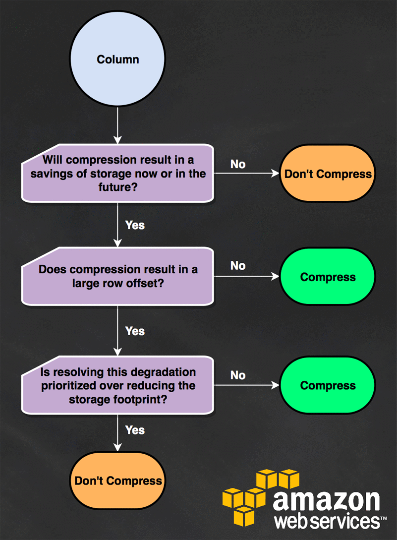
Now that I’ve convinced you, what compression to pick for your columns?

ANALYZE COMPRESSION TABLE_NAME_HERE;

The easiest way to determine the optimal compression is to finish designing the basics of your table, load sample data in, then utilize the ANALYZE COMPRESSION command (statement above, more on it here). Its output will tell you the compression that best works for your sample data for each column, thus doing all the work for you. From there, update your table definition and load the data again. Your disk size should now be smaller (disk size query provided in table metadata section).

Still not sure what to pick? Perhaps you don’t have data yet? Here’s an easy to remember rule of thumb:

• If it’s your sort key or a boolean, use RAW
• Otherwise, use ZSTD

That should get you started until you have enough data to go in and reviews compression choices, as ZSTD gives very strong compression across the majority of data types without a performance hit you’d notice.

More on compression here.

References to compression and performance can be found here, here, and here.

Distribution and sort

It is important to understand the difference between distribution of data and sort of data before moving on to how to use them to your advantage, as they can have the biggest impact on your table’s performance.

• Distribution of the data refers to which node it goes to.
• Sort of the data refers to where on the node it goes to.

If your distribution style is even, that means all nodes will get the same amount of data. Or if your distribution style is by key, each node will have data from the same one or more keys.

Once the node your data will live on is decided, the sort impacts its ordering there. If you have time sensitive data, you may want each node to store it in order of when it happened. As data comes in, it isn’t necessarily sorted right away (unsorted data discussed below) but it will be by Redshift as and when necessary or forced (such as during maintenance).

Distribution

There are two times when data is distributed:

1. When data is first inserted
2. When a query requires data for joins and aggregations

The second scenario is more important in terms of the performance impact, as having the data already where it needs to be for a query will have the biggest savings impact by allowing data to only be distributed in the first scenario without a redistribution that slows down the user’s query.

An ideal distribution of data allows each node to handle the same amount of work in parallel with minor amounts of redistribution. This is true both within a table and across tables: two tables constantly joined should have similar distributions so that the data needing joining is already present on the same node.

Using the most important and intensive query(ies) allows for the appropriate distribution style to be chosen (more on using the query plan for distribution decisions here), of which there are three options, ranked from least likely to be of use to you to most likely:

1. An ALL distribution puts a copy of the entire table on every node.
2. An EVEN distribution splits data up evenly across all nodes without looking at the content of the data.
   • This is helpful if you never join the table with other data or there is no clear way to leverage a KEY distribution (below).
3. A KEY distribution splits data up according to part of the data (the key).

Start by seeing if there’s a particular key that your query is dependent on. If there’s no obvious one or no joins with other tables, then consider an even distribution. In a staging environment, you can also try setting up the table multiple ways and experimenting with what would happen to get an idea of the impact of the different distribution styles.

More on data distribution here.

More on best practices here.

Sort

The sort of data can be leveraged in query execution, especially when there is a range of data being looked at: if the data is already sorted by range, then only that chunk of data needs to be used rather than picking up a larger number of smaller chunks of data. I now regret using the word “chunks” but we’re sticking with it.

There are two options for sorting and which one you pick is highly coupled with the query(ies) you will execute:

• A COMPOUND sort key uses a prefix of the sort keys’ values and can speed up JOIN, GROUP BY, ORDER BY, and compression.
  • The order of the keys matter.
  • The size of the unsorted region impacts the performance.
  • Use with increasing attributes like identities or datetimes over an INTERLEAVED key.
  • This is the default sort style.
• An INTERLEAVED sort key gives equal weight to all columns in the sort key and can improve performance when there are multiple queries with different filter criteria or heavily used secondary sort columns.
  • The order of the keys does not matter.
  • Performance of INTERLEAVED over COMPOUND may increase
    • As more sorted columns are filtered in the query.
    • If the single sort column has a long common prefix (think full URLs).

For what to put in the sort key, look at the query’s filter conditions. If you are constantly using a certain set of columns for equality checks or range checks, or you tend to look at data by slice of time, those columns should be leveraged in the sort. If you join your table to another table frequently, put the join column in the sort and distribution key to ensure local work.

Using EXPLAIN on a query against a table with sort keys established will show the impact of your sorting on the query’s execution.

More on data sorting here.

More on best practices here.

Table analysis

There are built in commands and tables that can be used to generate and view certain metadata about your table. To ease your burden, the following queries are provided for you premade.

More on the ANALYZE command here.

More on analyzing tables here.

Table schema

SELECT * FROM pg_table_def WHERE tablename = 'TABLE_NAME_HERE';

Table compression

ANALYZE COMPRESSION TABLE_NAME_HERE;

The results will tell you, for each column, what encoding is suggested and the size (in percentage) that would be saved by using that encoding over what is currently there.

Table metadata

ANALYZE VERBOSE SCHEMA_HERE.TABLE_NAME_HERE;
SELECT
    tableInfo.table AS tableName,
    results.endtime AS lastRan,
    results.status AS analysisStatus,
    results.rows AS numRows,
    tableInfo.unsorted AS percentUnsorted,
    tableInfo.size AS sizeOnDiskInMB,
    tableInfo.max_varchar AS maxVarCharColumn,
    tableInfo.encoded AS encodingDefinedAtLeastOnce,
    tableInfo.diststyle AS distStyle,
    tableInfo.sortkey_num AS numSortKeys,
    tableInfo.sortkey1 AS sortKeyFirstColumn
FROM SVV_TABLE_INFO AS tableInfo
LEFT JOIN STL_ANALYZE AS results
ON results.table_id = tableInfo.table_id
WHERE
    tableInfo.schema = 'SCHEMA_HERE'
    AND tableName = 'TABLE_NAME_HERE'
ORDER BY lastRan DESC
LIMIT 1;

This query has two parts: the first analyzes the table (VERBOSE here indicates that it updates you of its status as it runs) and the second outputs metadata from two system tables. The columns have been aliased for easier reading.

All columns in the SVV_TABLE_INFO table here.

All columns in the STL_ANALYZE table here.

Data loading

More on data loading here.

Unsorted data

As data comes into a node, it is not always efficient to sort it in right away. To see how much of a table is unsorted, you can leverage SVV_TABLE_INFO.unsorted from the above table metadata section. A smaller unsorted region means more data is exactly where you told the node it should be.

If data tends to come in slowly, regularly running VACUUM will clean up the unsorted region. This can be done as part of regular maintenance at a time when it will have the smallest impact on users.

If data tends to come in in large batches, see below for efficient bulk loading.

If data tends to be removed from the table wholesale, truncate instead of deleting the rows. TRUNCATE will clean up the disk space whereas DELETE does not.

More on managing the unsorted region here.

Efficient bulk loads

Some tips for all bulk loads:

• Load your data in sort key order.
• Do not do loads during maintenance windows.

From S3

Use the COPY command. You can even have it choose column compression for you.

More on loading from S3 here.

From another Redshift table

Use a bulk INSERT/SELECT command.

In a SQL statement

If the data is not yet available on any remote host, use a multirow INSERT command.

Debugging

What just happened?

You can query for queries that have been run in multiple ways:

• If you want all queries regardless of type, use the statement table.
• If you want all queries that were DDL, use the DDL table.
  • Eg create table, add column, etc
• If you want all queries that were DQL, use the query table.
  • Eg select, insert, update, delete, etc
• If you want all queries that are neither DDL nor DQL, use the utility table.
  • Eg grant, create user, commit, etc

InternalError: Load into table 'X' failed. Check 'stl_load_errors' system table for details.

It is recommended you to turn on \x to view this table.

SELECT
    errors.starttime,
    info.table,
    errors.colname,
    errors.err_reason,
    errors.raw_line
FROM stl_load_errors AS errors
LEFT JOIN SVV_TABLE_INFO AS info
ON errors.tbl = info.table_id
ORDER BY 1 DESC
LIMIT 5; --that’s just so you don’t get overwhelmed

Show all tables

SELECT schemaname, tablename FROM pg_table_def WHERE schemaname != 'pg_catalog' AND NOT tablename LIKE '%_pkey' ORDER BY schemaname, tablename;

Describe a table

SELECT * FROM pg_table_def WHERE schemaname = 'public' AND tablename = 'TABLE_NAME';

What are the largest tables?

SELECT
    tableInfo.schema AS schemaName,
    tableInfo.table AS tableName,
    tableInfo.unsorted AS percentUnsorted,
    tableInfo.size AS sizeOnDiskInMB
FROM svv_table_info AS tableInfo
ORDER BY sizeOnDiskInMB DESC
LIMIT 25;

Congratulations, you now have the GameChanger Data Engineering seal of approval for Redshift Basics!

As you work with Redshift, you’ll start to develop your own rules of thumb and opinions that might add on to what I’ve presented or differ from those rules of thumb we use here. And that’s ok! Redshift is an evolving system that is designed for many different use cases: there is no right design.

And remember, this isn’t everything there is to know about Redshift nor even all of the features it has for you to make use of. However this does cover the vast majority of basic use cases, and basic use cases are what you want to break your problems into. It’ll make your life easier, and your Redshift work easier too.